The basic language or R Markdown documents is (perhaps unsurprisingly) markdown. This is a markup language which allows a plain text file (not pointing or clicking) to be turned into amongst other things HTML. R Markdown extends this and adds things like R code chunks and certain elements of LaTeX to allow plain text documents to produce amongst other things Word, PDF, HTML documents, websites and books.
The bookdown package extends R Markdown and enables some more LaTeX functionality which is useful for scientific writing. It also easily facilitates the compilation of multiple R Markdown documents into a single final document. thesisdownrli has added a custom LaTeX template to build a pdf thesis out of R markdown chapters.
## Markdown
Most of an R Markdown file is made up of plain text. Small bits of markup change plain text into formatted text. Headings are preceded by a particular number of #
# Heading 1
## Heading 2
### Heading 3
#### Heading 4
##### Heading 5
It is also possible to add bold, italic etc:
-
_italic_or*italic*produces italic or italic -
__bold__or**italic**produces bold or bold -
R^2^produces R2 -
R~2~produces R2
Lists require at least one clear line break from the preceding paragraph.
1. item 1
2. item 2
  i. subitem i
  ii. subitem ii
3. item 3
would produce
- item 1
- item 2
  - subitem i
  - subitem ii
- item 3
or they can be unordered
- item 1
- item 2
- subitem i
- subitem ii
- item 3- item 1
- item 2
- subitem i
- subitem ii
- item 3
R
It is not necessary actually run any code from the thesis chapters but you have this option. To run code it needs to be enclosed in an R chunk. An example is shown below. Note the 3 backticks and r above the line of code and the 3 backticks to close. In this case the chunk is also named pressure. This name can be used to refer to the chunk, which is necessary for referencing figures - more information below.
```{r summary}
summary(cars)
```
speed dist
Min. : 4.0 Min. : 2.00
1st Qu.:12.0 1st Qu.: 26.00
Median :15.0 Median : 36.00
Mean :15.4 Mean : 42.98
3rd Qu.:19.0 3rd Qu.: 56.00
Max. :25.0 Max. :120.00 R can also be included inline as `r 2+2`. The code itself won’t be printed only the result of 4. This means variables (and their values) can be directly printed.
For example a value can be stored as part of some work:
```{r initial_props}
S_in = 0.99
I_in = 0.01
R_in = 0
```
We can then type something like:
The initial proportions of susceptible, infected and resistant individuals were
`r S_in`,`r I_in`and`r R_in`respectively.
Which would print out:
The initial proportions of susceptible, infected and resistant individuals were 0.99, 0.01 and 0 respectively.
Using values in text like this means that if for some reason the data changes slightly, it isn’t necessary to change all the values in text - they will change automatically the next the document is knitted.
Figures
Each plot produced from an R chunk will become a figure, with a caption if provided.
```{r chunk-name, fig.cap = "Scatterplot of Pressure", fig.height = 4, fig.width = 6}
plot(pressure)
```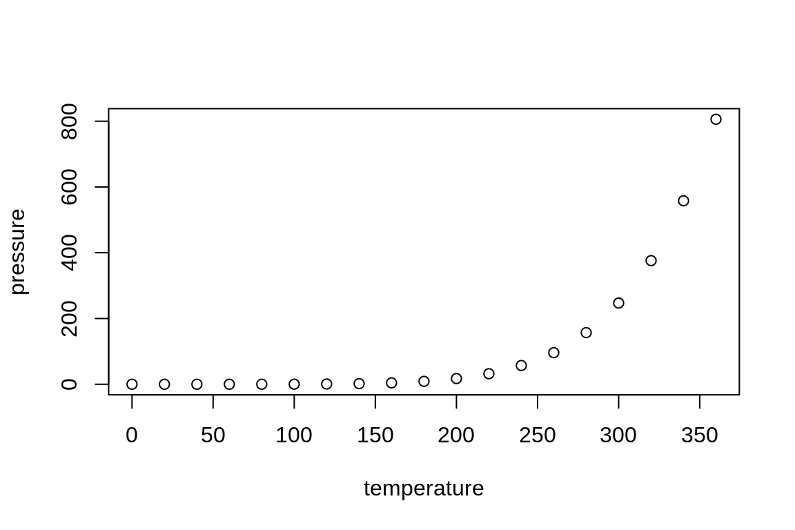
Scatterplot of Pressure
As the figure chunk has a name, this can be referenced using the syntax \@ref(fig:chunk-name). Note: Be careful to add the fig: before the chunk name here. For this to work the chunk name can only contain letters, numbers and dashes.
So in text we would have.
Figure
\@ref(fig:chunk-name)shows a scatterplot of pressure against temperature.
Images that haven’t been generated with directly from an R chunk or a source R file into an R markdown document. There are a couple of ways to do so but the best method for a thesis is to use a code chunk like the one below. A little bit of R code is used to include the graphics. Ideally the image should be in a subfolder.
```{r other-image, eval = FALSE}
knitr::include_graphics("path/to/file.png")
```
This method allows for figure captions and references to be used as above.
For all additional guidance on R plots and figures in bookdown please refer to the official documentation.
Equations
We can insert nicely formatted LaTeX equations in all R Markdown documents. An example would be
\begin{equation}
y = k e^{(\alpha - \beta)t}
\end{equation}
which would produce
and there are more examples below.
However, in order to add numbers to these equations and refer back to them we need to use the added functionality provided by bookdown. To do that we need add a label in the form (\#eq:equation-label). For example:
\begin{equation}
y = k e^{(\alpha - \beta)t}
(\#eq:example-eqn)
\end{equation}
which can be referenced using similar syntax as figures \@ref(eq:example-eqn).
As with figures for more detail please refer to the official bookdown documentation
A (Very) Brief Guide LaTeX Syntax
Below are some examples of how to use certain mathematical notation.
- Powers:
x^2would become \(x^2\). - Roots:
\sqrt{x}would become \(\sqrt{x}\). - Subscripts:
x_1would become \(x_1\). - Brackets
(x^2)would become \((x^2)\). If you want them to automatically become the correct size you can use\left(\frac{1}{2}\right)which will produce \(\left(\frac{1}{2}\right)\). - Greek letters:
\alpha,\beta,\delta,\epsilonand\gammawould become \(\alpha\), \(\beta\), \(\delta\), \(\epsilon\) and \(\gamma\). - Fractions:
\frac{3}{2}would become \[\frac{3}{2}\] - To get the normal derivative we use particular font:
\begin{equation}
\frac{\textrm{dy}}{\textrm{dx}} = x
\end{equation}- To align multiple equations we use the
\begin{align}environment where all the&will line up and we indicate a new line with\\. Don’t put a new line after the last equation.
\begin{align}
\frac{\textrm{dy}_1}{\textrm{dx}} &= x \\
\frac{\textrm{dy}_2}{\textrm{dx}} &= x \\
\frac{\textrm{dy}_3}{\textrm{dx}} &= x
\end{align}